Galaxy-galaxy simulations

This notebook walks through the basics of simulating a galaxy-galaxy strong lensing population. The underlying assumptions of the galaxy populations (for both lenses and sources) are drawn from a population pre-configured and rendered through SkyPy. The specific settings are described in the readme file.

The notebook goes in three steps:

1. The populations of lenses and sources is produced.

2. Random draws of the population are generated and realized as images

3. The full population is generated in catalogue form

4. the full population is represented in a corner plot

Generate population of galaxies and (potential) deflectors

The LensPop() class in the slsim package is used to produce a set of galaxies (as lenses and sources)

as seen on the sky within a certain sky area. We use the default SkyPy configuration file. Alternative configuration

files can be used.

import matplotlib.pyplot as plt
from astropy.cosmology import FlatLambdaCDM
from astropy.units import Quantity
from slsim.lens_pop import LensPop
from slsim.Plots.lens_plots import LensingPlots
import numpy as np
import corner

# define a cosmology
cosmo = FlatLambdaCDM(H0=70, Om0=0.3)

# define a sky area
sky_area = Quantity(value=0.1, unit="deg2")


# define limits in the intrinsic deflector and source population (in addition to the skypy config
# file)
kwargs_deflector_cut = {"band": "g", "band_max": 28, "z_min": 0.01, "z_max": 2.5}
kwargs_source_cut = {"band": "g", "band_max": 28, "z_min": 0.1, "z_max": 5.0}

# run skypy pipeline and make galaxy-galaxy population class using LensPop
gg_lens_pop = LensPop(
    deflector_type="all-galaxies",
    source_type="galaxies",
    kwargs_deflector_cut=kwargs_deflector_cut,
    kwargs_source_cut=kwargs_source_cut,
    kwargs_mass2light=None,
    skypy_config=None,
    sky_area=sky_area,
    cosmo=cosmo,
)

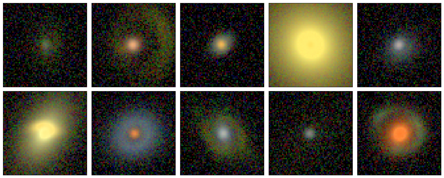
Generate images of random lenses

The LensingPlots() class has the functionality to draw random lenses and makes an image of it. Currently

default settings in lenstronomy are chosen for the LSST image settings. These will be able to be replaced with the

LSST simulation tools.

# make some cuts in the image separations and limited magnitudes of the arc
kwargs_lens_cut_plot = {
    "min_image_separation": 0.8,
    "max_image_separation": 10,
    "mag_arc_limit": {"g": 23, "r": 23, "i": 23},
}


gg_plot = LensingPlots(gg_lens_pop, num_pix=64, coadd_years=10)

# generate montage indicating which bands are used for the rgb color image
fig, axes = gg_plot.plot_montage(
    rgb_band_list=["i", "r", "g"],
    add_noise=True,
    n_horizont=5,
    n_vertical=2,
    kwargs_lens_cut=kwargs_lens_cut_plot,
)
plt.show()

Generate the full population

We are using the instance of the LensPop() class to draw the full population within specified cuts in a Monte Carlo process.

# specifying cuts of the population
kwargs_lens_cuts = {"mag_arc_limit": {"g": 28}}
# drawing population
gg_lens_population = gg_lens_pop.draw_population(kwargs_lens_cuts=kwargs_lens_cuts)

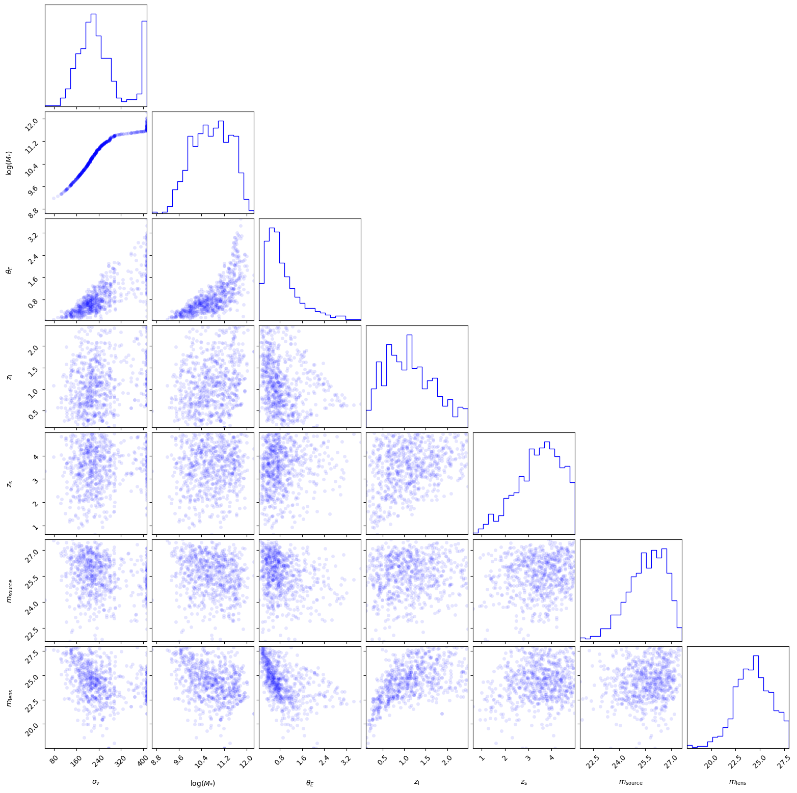
Represent key quantities of full population in corner plots

We calculate few key quantities of the lenses. The full population is represented each with a Lens() class

object that allows to compute and return these (and more) quantities.

print("Number of lenses:", len(gg_lens_population))

lens_samples = []
labels = [
    r"$\sigma_v$",
    r"$\log(M_{*})$",
    r"$\theta_E$",
    r"$z_{\rm l}$",
    r"$z_{\rm s}$",
    r"$m_{\rm source}$",
    r"$m_{\rm lens}$",
]

for gg_lens in gg_lens_population:
    vel_disp = gg_lens.deflector_velocity_dispersion()
    m_star = gg_lens.deflector_stellar_mass()
    theta_e = gg_lens.einstein_radius
    zl = gg_lens.deflector_redshift
    zs = gg_lens.source_redshift
    source_mag = gg_lens.extended_source_magnitude(band="g", lensed=True)
    deflector_mag = gg_lens.deflector_magnitude(band="g")
    lens_samples.append(
        [vel_disp, np.log10(m_star), theta_e, zl, zs, source_mag, deflector_mag]
    )

Number of lenses: 686

hist2dkwargs = {
    "plot_density": False,
    "plot_contours": False,
    "plot_datapoints": True,
    "color": "b",
    "data_kwargs": {"ms": 5},
}
corner.corner(np.array(lens_samples), labels=labels, **hist2dkwargs)
plt.show()